@axis
-모든 operation funtion을 실행할 때, 기준이 되는 dimension 축
import numpy as np

print(np.arange(1, 13).reshape(3, 4))
output)
[[ 1  2  3  4]
 [ 5  6  7  8]
 [ 9 10 11 12]]

-처음 생기는 shape은 항상 0
그 후로 shape이 생기면 하나씩 뒤로 밀려 항상 새로 생기는 shape이 0, 기존의 shape은 1이 됨
import numpy as np
test_array = np.arange(1, 13).reshape(3, 4)
print(test_array.sum(axis=1))
output)

[10 26 42]-axis=1 : column(열) 기준으로 더하라
import numpy as np
test_array = np.arange(1, 13).reshape(3, 4)
print(test_array.sum(axis=0))
output)
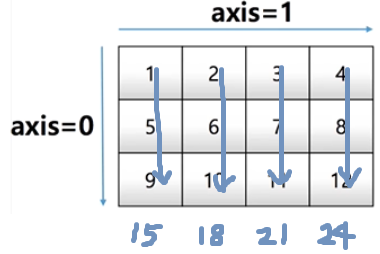
[15 18 21 24]-axis=0 : row(행) 기준으로 더하라
*그냥 sum을 하면 해당 array에 있는 모든 element를 더해줌
@concatenate(쉽게 말하면 붙이는 것)
-Numpy array를 합치는 함수

import numpy as np

test_a = np.array([1, 2, 3])
test_b = np.array([4, 5, 6])
print(np.vstack((test_a, test_b)))
output)
[[1 2 3]
 [4 5 6]]

import numpy as np

test_a = np.array([[1], [2], [3]])
test_b = np.array([[4], [5], [6]])
print(np.hstack((test_a, test_b)))
output)
[[1 4]
 [2 5]
 [3 6]]
번외)
import numpy as np

test_a = np.array([1, 2, 3])
test_b = np.array([4, 5, 6])
print(np.hstack((test_a, test_b)))
output)
[1 2 3 4 5 6]test_a = np.array([1, 2, 3])
test_b = np.array([4, 5, 6])
이렇게 했더니 일렬로 다 붙여지넹
Using concatenate funtion>

import numpy as np

test_a = np.array([[1, 2, 3]])
test_b = np.array([[4, 5, 6]])
print(np.concatenate((test_a, test_b), axis=0))
output)
[[1 2 3]
 [4 5 6]]
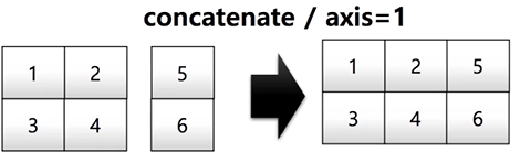
import numpy as np

test_a = np.array([[1, 2], [3, 4]])
test_b = np.array([[5, 6]])
print(np.concatenate((test_a, test_b.T), axis=1))
output)
[[1 2 5]
 [3 4 6]]
@Operations b/t arrays
-Numpy는 array간 기본적인 사칙 연산 지원
-vector간 계산이나 matrix간 계산을 간단히 수행 가능
*Matrix내 element들 간 같은 위치에 있는 값들끼리 연산
Mat + Mat
import numpy as np

test_a = np.array([[1, 2, 3], [4, 5, 6]], float)
print(test_a + test_a)
output)
[[ 2.  4.  6.]
 [ 8. 10. 12.]]
Mat - Mat
import numpy as np

test_a = np.array([[1, 2, 3], [4, 5, 6]], float)
print(test_a - test_a)
output)
[[0. 0. 0.]
 [0. 0. 0.]]
Mat * Mat
import numpy as np

test_a = np.array([[1, 2, 3], [4, 5, 6]], float)
print(test_a * test_a)
output)
[[ 1.  4.  9.]
 [16. 25. 36.]]
@Element-wise operations

-Array 간 shape이 같을 때 일어나는 연산
import numpy as np

test_a = np.arange(1, 13).reshape(3, 4)
print(test_a * test_a)
output)
[[  1   4   9  16]
 [ 25  36  49  64]
 [ 81 100 121 144]]
@Dot product

-Matrix의 기본 연산
-dot 함수 사용
import numpy as np

test_a = np.arange(1, 7).reshape(2, 3)
test_b = np.arange(7, 13).reshape(3, 2)

print(test_a.dot(test_b))
output)
[[ 58  64]
 [139 154]]
@transpose(전치행렬)
-transpose 또는 T attribute 사용
import numpy as np

test_a = np.arange(1, 7).reshape(2, 3)
print(test_a)

print(test_a.transpose())
print(test_a.T)
output)
# test_a
[[1 2 3]
 [4 5 6]]
# test_a.transpose()
[[1 4]
 [2 5]
 [3 6]]
# test_a.T
[[1 4]
 [2 5]
 [3 6]]
Matrix 간 곱셈
import numpy as np

test_a = np.arange(1, 7).reshape(2, 3)
print(test_a)

print(test_a.T.dot(test_a))
output)
# test_a
[[1 2 3]
 [4 5 6]]
# test_a.T.dot(test_a)
[[17 22 27]
 [22 29 36]
 [27 36 45]]
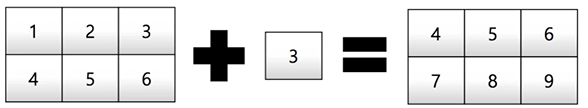
@broadcasting
-Numpy는 broadcasting을 일으킴
-Shape이 다른 배열 간 연산을 지원하는 기능
-가장 많이 이용될 때는 Matrix와 Scalar 간 연산
import numpy as np

test_matrix = np.array([[1,2,3],[4,5,6]], float)
scalar = 3

print(test_matrix + scalar)
print(test_matrix - scalar)
print(test_matrix * 5)
print(test_matrix / 5)
print(test_matrix // 0.2)
print(test_matrix ** 2)
output)
# test_matrix + scalar
[[4. 5. 6.]
 [7. 8. 9.]]
# test_matrix - scalar
[[-2. -1.  0.]
 [ 1.  2.  3.]]
# test_matrix * 5
[[ 5. 10. 15.]
 [20. 25. 30.]]
# test_matrix / 5
[[0.2 0.4 0.6]
 [0.8 1.  1.2]]
# test_matrix // 0.2
[[ 4.  9. 14.]
 [19. 24. 29.]]
# test_matrix ** 2
[[ 1.  4.  9.]
 [16. 25. 36.]]
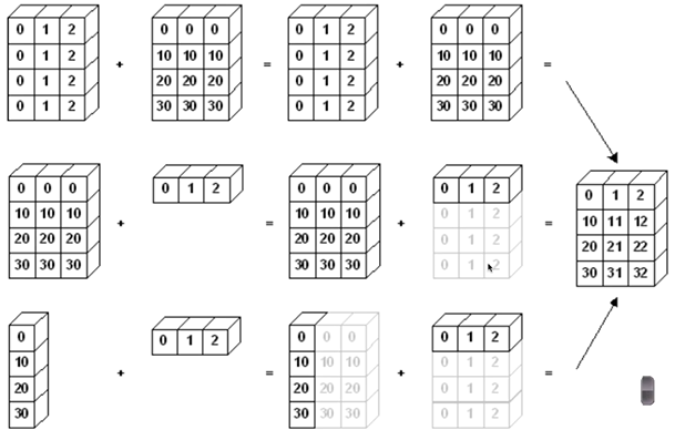
-broadcasting은 Scalar-Vector 외에도 Vector-Matrix 간 연산도 지원
'CS > Python' 카테고리의 다른 글
| Numpy data i/o (0) | 2021.02.20 |
|---|---|
| Numerical Python - Numpy(3) (0) | 2021.02.20 |
| Numerical Python - Numpy(1) (0) | 2021.02.18 |
| PCA: How to use in Python (0) | 2021.02.08 |
| Basic Linear Algebra | 선형대수 기본 (0) | 2021.01.18 |


