너무 길어서 수식 쓰기 어려울 때 matrix 도입
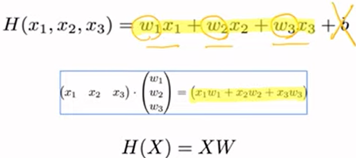
뒤에 있는 상수는 문제 쉽게 풀기 위해 제외하고 진행
스칼라 곱은 동일한 결과값 가짐(순서 바뀌어도 ㄱㅊ)
WX와 XW 동일한 표현
- Theory
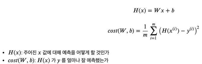
H(x) = Wx + b
- Implementation
H(X) = XW
@pytorch
-Torch 라는 딥러닝/머신러닝 라이브러리에 해당
-> python으로 사용할 수 있도록 warpping한 언어
-Torch라는 언어 사용해서 프로그래밍 해야하지만 python 으로도 가능
- linear_regression.py
# -*- coding: utf-8 -*-
"""linear_regression.ipynb

Automatically generated by Colaboratory.

You can check the ipynb code at
    https://github.com/iamdami/Python_Practice/blob/main/SEJONG_prof_Choi/linear_regression.ipynb
"""

import torch
import torch.optim as optim
# 다양한 최적화 알고리즘 구현해 놓은 패키지

torch.manual_seed(1)
# seed 함수 호출해 고정
# seed 고정해 놓으면 매번 랜덤함수 호출 시 동일한 값 호출

"""#Data"""

# (x1, y1)=(1, 1), (x2, y2)=(2, 2), (x3, y3)=(3, 3)
x_train = torch.FloatTensor([[1], [2], [3]])
y_train = torch.FloatTensor([[1], [2], [3]])

print(x_train)
print(x_train.shape)

print(y_train)
print(y_train.shape)

"""# Weight Initialization"""

W = torch.zeros(1, requires_grad=True)  # 학습용 변수 선언
print(W)

b = torch.zeros(1, requires_grad=True)
print(b)

"""# Hypothesis"""

hypothesis = x_train * W + b
print(hypothesis)

"""# Cost"""

print(hypothesis)

print(y_train)

print(hypothesis - y_train)

print((hypothesis - y_train) ** 2)

cost = torch.mean((hypothesis - y_train) ** 2)
print(cost)

"""# Gradient Descent"""

# learning rate -> lr = 0.01
# W := W - alpha * d / dw * cost(w)
optimizer = optim.SGD([W, b], lr = 0.01)

# 옵티마이저 계산
optimizer.zero_grad()
# cost 계산
cost.backward()
# 옵티마이저 갱신
optimizer.step()

print(W)
print(b)

"""check if the hypothesis get better"""

hypothesis = x_train * W + b
print(hypothesis)

cost = torch.mean((hypothesis - y_train) ** 2)
print(cost)

# data
x_train = torch.FloatTensor([[1], [2], [3]])
y_train = torch.FloatTensor([[1], [2], [3]])

# 모델 초기화
W = torch.zeros(1, requires_grad= True)
b = torch.zeros(1, requires_grad= True)

# 옵티마이저 설정
optimizer = optim.SGD([W, b], lr = 0.01)

nb_epochs = 1000
for epoch in range(nb_epochs + 1):

  # H(x) 계산
  hypothesis = x_train * W + b

  # cost 계산
  cost = torch.mean((hypothesis - y_train) ** 2)

  # cost로 H(x) 계산
  optimizer.zero_grad()
  cost.backward()
  optimizer.step()

  # 100번마다 로그 출력
  if epoch % 100 == 0:
    print('Epoch {:4d} / {} W: {:.3f}, b: {:.3f} Cost: {:.6f}'.format(
        epoch, nb_epochs, W.item(), b.item(), cost.item()
    ))
- MinimizingCost.py
# -*- coding: utf-8 -*-
"""MinimizingCost.ipynb
Automatically generated by Colaboratory.
You can check the ipynb file code at
https://github.com/iamdami/Python_Practice/blob/main/SEJONG_prof_Choi/MinimizingCost.ipynb
# Imports
"""
import matplotlib.pyplot as plt # 시각화용 라이브러리
import numpy as np
import torch
import torch.optim as optim
torch.manual_seed(1)
"""# Data"""
x_train = torch.FloatTensor([[1], [2], [3]])
y_train = torch.FloatTensor([[1], [2], [3]])
plt.scatter(x_train, y_train)
# Best-fit line
xs = np.linspace(1, 3, 1000)
plt.plot(xs, xs)
print(xs)
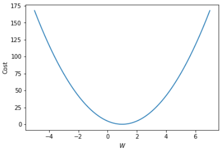
"""# Cost by W"""
# -5 ~ 7 사이를 1000등분
W_l = np.linspace(-5, 7, 1000)
cost_l = []
for W in W_l:
hypothesis = W * x_train
cost = torch.mean((hypothesis - y_train) ** 2)
cost_l.append(cost.item())
plt.plot(W_l, cost_l)
plt.xlabel('$W$')
plt.ylabel('Cost')
plt.show()
"""# Gradient Descent by Hand"""
W = 0
gradient = torch.sum((W * x_train - y_train) * x_train)
print(gradient)
lr = 0.1
W -= lr * gradient
print(W) # W 갱신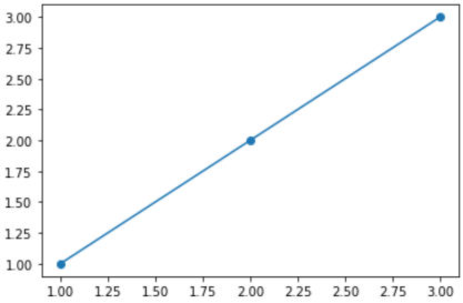
- Multivariable_linear_regression.py
# -*- coding: utf-8 -*-
"""Multivariable_linear_regression.ipynb

Automatically generated by Colaboratory.

You can check the ipynb file code at
    https://github.com/iamdami/Python_Practice/blob/main/SEJONG_prof_Choi/Multivariable_linear_regression.ipynb

# Imports
"""

import torch
import torch.optim as optim

torch.manual_seed(1)

"""# Naive Data Representation"""

# data
x1_train = torch.FloatTensor([[73], [93], [89], [96], [73]])
x2_train = torch.FloatTensor([[80], [88], [91], [98], [66]])
x3_train = torch.FloatTensor([[75], [93], [90], [100], [70]])
y_train = torch.FloatTensor([[152], [185], [180], [196], [142]])

# 모델 초기화
w1 = torch.zeros(1, requires_grad=True)
w2 = torch.zeros(1, requires_grad=True)
w3 = torch.zeros(1, requires_grad=True)
b = torch.zeros(1, requires_grad=True)

# 옵티마이저 설정
optimizer = optim.SGD([w1, w2, w3, b], lr = 0.00001)

nb_epochs = 1000
for epoch in range(nb_epochs + 1):

  # H(x) 계산
  hypothesis = x1_train * w1 + x2_train * w2 + x3_train * w3 + b

  # cost 계산
  cost = torch.mean((hypothesis - y_train) ** 2)

  # cost로 H(x) 개선
  optimizer.zero_grad()
  cost.backward()
  optimizer.step()

  # 100번마다 로그 출력
  if epoch % 100 == 0:
    print('Epoch {:4d} / {} w1: {:.3f} w2: {:.3f} w3: {:.3f} b: {:.3f} Cost: {:.6f}'.format(
        epoch, nb_epochs, w1.item(), w2.item(), w3.item(), b.item(), cost.item()
    ))

"""# Matrix Data Representation"""

x_train = torch.FloatTensor([[73, 80, 75],
                             [93, 88, 93],
                             [89, 91, 90],
                             [96, 98, 100],
                             [73, 66, 70]])
y_train = torch.FloatTensor([[152], [185], [180], [196], [142]])

print(x_train.shape)
print(y_train.shape)

# 모델 초기화
W = torch.zeros((3, 1), requires_grad=True)
b = torch.zeros(1, requires_grad=True)

# 옵티마이저 설정
optimizer = optim.SGD([W, b], lr = 0.00001)

nb_epochs = 20
for epoch in range(nb_epochs + 1):

  # H(x) 계산
  hypothesis = x_train.matmul(W) + b

  # cost 계산
  cost = torch.mean((hypothesis - y_train) ** 2)

  # cost로 H(x) 개선
  optimizer.zero_grad()
  cost.backward()
  optimizer.step()

  # 100번마다 로그 출력
  print('Epoch {:4d} / {} hypothesis: {} Cost: {:.6f}'.format(
      epoch, nb_epochs, hypothesis.squeeze().detach(), cost.item()
  ))
참고)
세종대 최유경 교수님 인공지능 강의
'CS > AI | CV' 카테고리의 다른 글
| 선형 분류 (0) | 2021.09.06 |
|---|---|
| 머신러닝 프로젝트 계획 (0) | 2021.08.31 |
| ID Photo Generator | 증명사진 생성기 (0) | 2021.07.26 |
| Semantic Segmentation, Instance Segmentation, Object detection (0) | 2021.07.23 |
| Active contour model (0) | 2021.07.22 |


